4. Digital Modulation

In this chapter we will discuss actually transmitting data using digital modulation and wireless symbols! We will design signals that convey “information”, e.g., 1’s and 0’s, using modulation schemes like ASK, PSK, QAM, and FSK. We will also discuss IQ plots and constellations, and end the chapter with some Python examples.

The main goal of modulation is to squeeze as much data into the least amount of spectrum possible. Technically speaking we want to maximize “spectral efficiency” in units bits/sec/Hz. Transmitting 1’s and 0’s faster will increase the bandwidth of our signal (recall Fourier properties), which means more spectrum is used. We will also examine other techniques besides transmitting faster. There will be many trade-offs when deciding how to modulate, but there will also be room for creativity.

Symbols

New term alert! Our transmit signal is going to be made up of “symbols”. Each symbol will carry some number of bits of information, and we will transmit symbols back to back, thousands or even millions in a row.

As a simplified example, let’s say we have a wire and are sending 1’s and 0’s using high and low voltage levels. A symbol is one of those 1’s or 0’s:

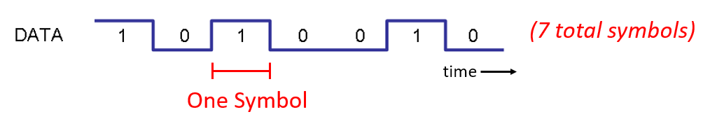
In the above example each symbol represents one bit. How can we convey more than one bit per symbol? Let’s study the signals that travel down Ethernet cables, which is defined in an IEEE standard called IEEE 802.3 1000BASE-T. The common operating mode of Ethernet uses a 4-level amplitude modulation (2 bits per symbol) with 8 ns symbols.

Take a moment to try to answer these questions:

1. How many bits per second are transmitted in the example shown above?

2. How many pairs of these data wires would be needed to transmit 1 gigabit/sec?

3. If a modulation scheme has 16 different levels, how many bits per symbol is that?

4. With 16 different levels and 8 ns symbols, how many bits per second is that?

Answers

1. 250 Mbps - (1/8e-9)*2

2. Four (which is what Ethernet cables have)

3. 4 bits per symbol - log_2(16)

4. 0.5 Gbps - (1/8e-9)*4

Wireless Symbols

Question: Why can’t we directly transmit the Ethernet signal shown in the figure above? There are many reasons, the biggest two being:

1. Low frequencies require huge antennas, and the signal above contains frequencies down to DC (0 Hz). We can’t transmit DC.

2. Square waves take an excessive amount of spectrum for the bits per second–recall from the Frequency Domain chapter that sharp changes in time domain use a large amount of bandwidth/spectrum:

What we do for wireless signals is start with a carrier, which is just a sinusoid. E.g., FM radio uses a carrier like 101.1 MHz or 100.3 MHz. We modulate that carrier in some way (there are many). For FM radio it’s an analog modulation, not digital, but it’s the same concept as digital modulation.

In what ways can we modulate the carrier? Another way to ask the same question: what are the different properties of a sinusoid?

1. Amplitude

2. Phase

3. Frequency

We can modulate our data onto a carrier by modifying any one (or more) of these three.

Amplitude Shift Keying (ASK)

Amplitude Shift Keying (ASK) is the first digital modulation scheme we will discuss because amplitude modulation is the simplest to visualize of the three sinusoid properties. We literally modulate the amplitude of the carrier. Here is an example of 2-level ASK, called 2-ASK:

Note how the average value is zero; we always prefer this whenever possible.

We can use more than two levels, allowing for more bits per symbol. Below shows an example of 4-ASK (off is one of the four levels). In this case each symbol carries 2 bits of information.

Question: How many symbols are shown in the signal snippet above? How many bits are represented total?

Answers

20 symbols, so 40 bits of information

How do we actually create this signal digitally, through code? All we have to do is create a vector with N samples per symbol, then multiply that vector by a sinusoid. This modulates the signal onto a carrier (the sinusoid acts as that carrier). The example below shows 2-ASK with 10 samples per symbol.

The top plot shows the discrete samples represented by red dots, i.e., our digital signal. The bottom plot shows what the resulting modulated signal looks like, which could be transmitted over the air. In real systems, the frequency of the carrier is usually much much higher than the rate the symbols are changing. In this example there are only 2.5 cycles of the sinusoid in each symbol, but in practice there may be thousands, depending on how high in the spectrum the signal is being transmitted. For more information on ASK we recommend this resource.

Phase Shift Keying (PSK)

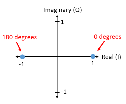
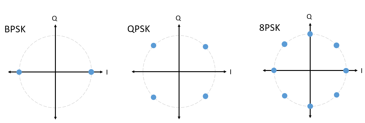
Now let’s consider modulating the phase in a similar manner as we did with the amplitude. The simplest form is Binary PSK, a.k.a. BPSK, where there are two levels of phase:

1. No phase change

2. 180 degree phase change

Example of BPSK (note the phase changes):

It’s not very fun to look at plots like this:

Instead we usually represent the phase in the complex plane.

IQ Plots/Constellations

You have seen IQ plots before in the complex numbers subsection of the IQ Sampling chapter, but now we will use them in a new and fun way. For a given symbol, we can show the amplitude and phase on an IQ plot. For the BPSK example we said we had phases of 0 and 180 degrees. Let’s plot those two points on the IQ plot. We will assume a magnitude of 1. In practice it doesn’t really matter what magnitude you use; a higher value means a higher power signal, but you can also just increase the amplifier gain instead.

The above IQ plot shows what we will transmit, or rather the set of symbols we will transmit from. It does not show the carrier, so you can think about it as representing the symbols at baseband. When we show the set of possible symbols for a given modulation scheme, we call it the “constellation”. Many modulation schemes can be defined by their constellation.

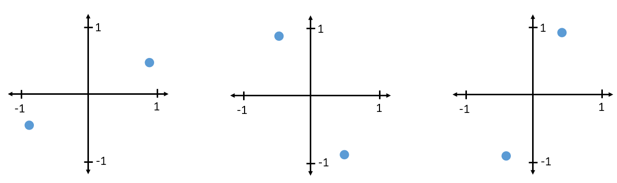
To receive and decode BPSK we can use IQ sampling, like we learned about last chapter, and examine where the points end up on the IQ plot. However, there will be a random phase rotation due to the wireless channel because the signal will have some random delay as it passes through the air between antennas. The random phase rotation can be reversed using various methods we will learn about later. Here is an example of a few different ways that BPSK signal might show up at the receiver (this does not include noise):

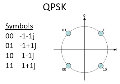
Back to PSK. What if we want four different levels of phase? I.e., 0, 90, 180, and 270 degrees. In this case it would be represented like so on the IQ plot, and it forms a modulation scheme we call Quadrature Phase Shift Keying (QPSK):

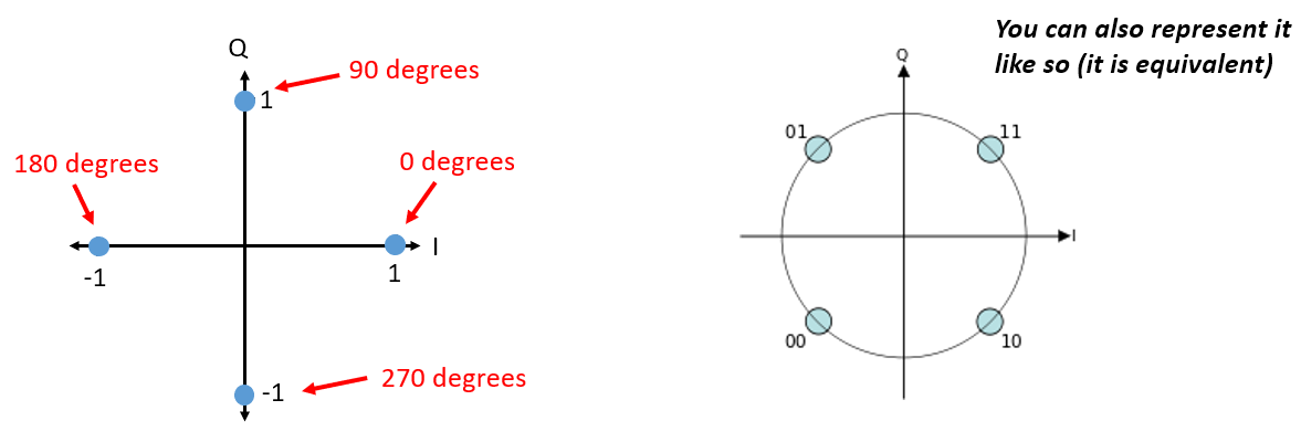
For PSK we always have N different phases, equally spaced around 360 degrees for best results. We often show the unit circle to emphasize that all points have the same magnitude:

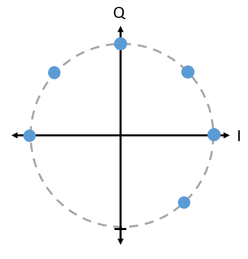
Question: What’s wrong with using a PSK scheme like the one in the below image? Is it a valid PSK modulation scheme?

Answer

There is nothing invalid about this PSK scheme. You can certainly use it, but, because the symbols are not uniformly spaced, this scheme is not as effective as it could be. Scheme efficiency will become clear once we discuss how noise impacts our symbols. The short answer is that we want to leave as much room as possible in between the symbols, in case there is noise, so that a symbol is not interpreted at the receiver as one of the other (incorrect) symbols. We don’t want a 0 being received as a 1.

Let’s detour back to ASK for a moment. Note that we can show ASK on the IQ plot just like PSK. Here is the IQ plot of 2-ASK, 4-ASK, and 8-ASK, in the bipolar configuration, as well as 2-ASK and 4-ASK in the unipolar configuration. In this context, bipolar means the modulated signal can take on both positive and negative amplitude values, whereas unipolar ASK only uses positive amplitudes.

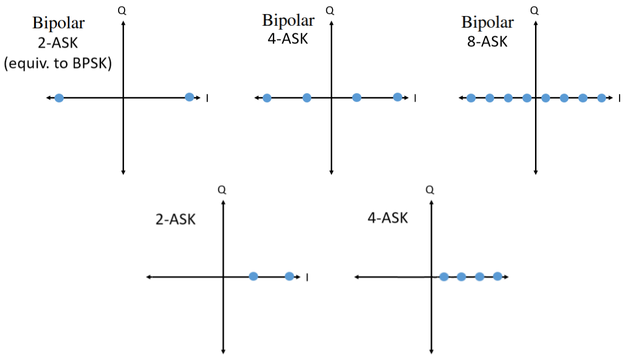
As you may have noticed, bipolar 2-ASK and BPSK are the same. A 180 degree phase shift is the same as multiplying the sinusoid by -1. We call it BPSK, probably because PSK is used way more than ASK.

Quadrature Amplitude Modulation (QAM)

What if we combine ASK and PSK? We call this modulation scheme Quadrature Amplitude Modulation (QAM). QAM usually looks something like this:

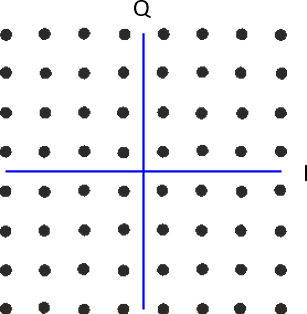
Here are some other examples of QAM:

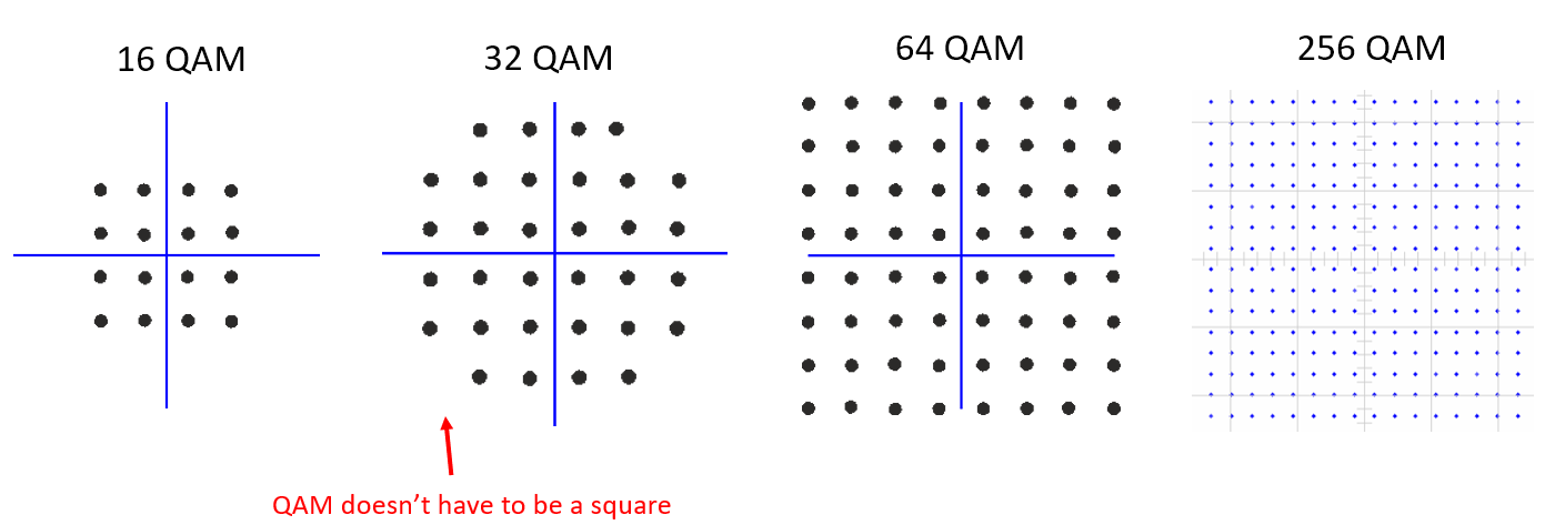
For a QAM modulation scheme, we can technically put points wherever we want to on the IQ plot since the phase and amplitude are modulated. The “parameters” of a given QAM scheme are best defined by showing the QAM constellation. Alternatively, you may list the I and Q values for each point, like below for QPSK:

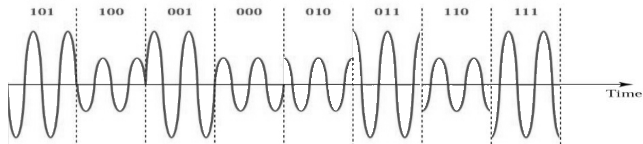
Note that most modulation schemes, except the various ASKs and BPSK, are pretty hard to “see” in the time domain. To prove my point, here is an example of QAM in time domain. Can you distinguish between the phase of each symbol in the below image? It’s tough.

Given the difficulty discerning modulation schemes in the time domain, we prefer to use IQ plots over displaying the time domain signal. We might, nonetheless, show the time domain signal if there’s a certain packet structure or the sequence of symbols matters.

Frequency Shift Keying (FSK)

Last on the list is Frequency Shift Keying (FSK). FSK is fairly simple to understand–we just shift between N frequencies where each frequency is one possible symbol. However, because we are modulating a carrier, it’s really our carrier frequency +/- these N frequencies. E.g.. we might be at a carrier of 1.2 GHz and shift between these four frequencies:

1. 1.2001 GHz

2. 1.2003 GHz

3. 1.1999 GHz

4. 1.1997 GHz

The example above would be 4-FSK, so there would be two bits per symbol. The frequency spacing is 200 kHz, and the total signal would span slightly more than 600 kHz. This 4-FSK signal in the frequency domain at baseband might look something like this, when doing an FFT over many symbols:

If you use FSK, you must ask a critical question: What should the spacing between frequencies be? We often denote this spacing as \(\Delta f\) in Hz. We want to avoid overlap in the frequency domain so that the receiver knows which frequency a given symbol used, so \(\Delta f\) must be large enough. The width of each carrier in frequency is a function of our symbol rate and any pulse shaping filter applied. More symbols per second means shorter symbols, which means wider bandwidth (recall the inverse relationship between time and frequency scaling). The faster we transmit symbols, the wider each carrier will get, and consequently the larger we have to make \(\Delta f\) to avoid overlapping carriers.

IQ plots can’t be used to show different frequencies. They show magnitude and phase. While it is possible to show FSK in the time domain, any more than 2 frequencies makes it difficult to distinguish between symbols:

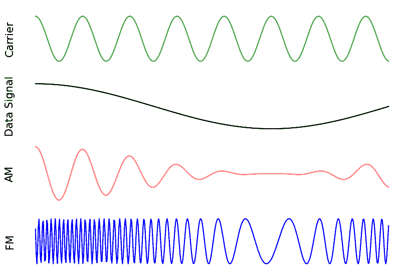
As an aside, note that FM radio uses Frequency Modulation (FM) which is like an analog version of FSK. Instead of having discrete frequencies we jump between, FM radio uses a continuous audio signal to modulate the frequency of the carrier. Below is an example of FM and AM modulation where the “signal” at the top is the audio signal being modulated onto to the carrier.

In this textbook we are mainly concerned about digital forms of modulation.

Differential Coding

In many wireless (and wired) communications protocols based on PSK or QAM, you are likely to run into a step that occurs right before bits are modulated (or right after demodulation), called differential coding. To demonstrate its utility consider receiving a BPSK signal. As the signal flies through the air it experiences some random delay between the transmitter and receiver, causing a random rotation in the constellation, as we mentioned earlier. When the receiver synchronizes to it, and aligns the BPSK to the “I” (real) axis, it has no way of knowing if it is 180 degrees out of phase or not, because the constellation is symmetric. One option is to transmit symbols the receiver knows the value of ahead of time, mixed into the information, known as pilot symbols. The receiver can use these known symbols to determine which cluster is a 1 or 0, in the case of BPSK. Pilot symbols must be sent at some period, related to how fast the wireless channel is changing, which will ultimately reduce the data rate. Instead of having to mix pilot symbols into the transmitted waveform, we can choose to use differential coding.

The simplest case of differential coding is when used alongside BPSK, which involves one bit per symbol. Instead of simply transmitting a 1 for binary 1, and a -1 for binary 0, BPSK differential coding involves transmitting a 0 when the input bit is the same as the encoding of the previous bit (not the previous input bit itself), and transmitting a 1 when it differs. We still transmit the same number of bits, aside from one extra bit that is needed at the beginning to start the output sequence, but now we don’t have to worry about the 180 degree phase ambiguity. This encoding scheme can be described using the following equation, where \(x\) are the input bits and \(y\) are the output bits that will get modulated with BPSK:

\[y_i = y_{i-1} \oplus x_i\]

Because the output is based on the previous step’s output, we must start the output with an arbitrary 1 or 0, and as we’ll show during the decoding process, it doesn’t matter which one we choose (we must still transmit this starter symbol!).

For those visual learners, the differential encoding process can be represented as a diagram, where the delay block is a delay-by-1 operation:

As an example of encoding, consider transmitting the 10 bits [1, 1, 0, 0, 1, 1, 1, 1, 1, 0] using BPSK. Assume we start the output sequence with 1; it actually doesn’t matter whether you use 1 or 0. It helps to show the bits stacked on top of each other, making sure to shift the input to make room for the starting output bit:

Input:     1 1 0 0 1 1 1 1 1 0
Output:  1

Next you build the output by comparing the input bit with the previous output bit, and apply the XOR operation shown in the table above. The next output bit is therefore a 0, because 1 and 1 match:

Input:     1 1 0 0 1 1 1 1 1 0
Output:  1 0

Repeat for the rest and you will get:

Input:     1 1 0 0 1 1 1 1 1 0
Output:  1 0 1 1 1 0 1 0 1 0 0

After applying differential encoding, we would ultimately transmit [1, 0, 1, 1, 1, 0, 1, 0, 1, 0, 0]. The 1’s and 0’s are still mapped to the positive and negative symbols we discussed earlier.

The decoding process, which occurs at the receiver, compares the received bit with the previous received bit, which is much simpler to understand:

\[x_i = y_i \oplus y_{i-1}\]

If you were to receive the BPSK symbols [1, 0, 1, 1, 1, 0, 1, 0, 1, 0, 0], you would start at the left and check if the first two match; in this case they don’t so the first bit is a 1. Repeat and you will get the sequence we started with, [1, 1, 0, 0, 1, 1, 1, 1, 1, 0]. It may not be obvious, but the starter bit we added could have been a 1 or a 0 and we would get the same result.

The encoding and decoding process is summarized in the following graphic:

The big downside to using differential coding is that if you have a bit error, it will lead to two bit errors. The alternative to using differential coding for BPSK is to add pilot symbols periodically, as discussed earlier, which can also be used to reverse/invert multipath caused by the channel. But one problem with pilot symbols is that the wireless channel can change very quickly, on the order of tens or hundreds of symbols if it’s a moving receiver and/or transmitter, so you would need pilot symbols often enough to reflect the changing channel. So if a wireless protocol is putting high emphasis on reducing the complexity of the receiver, such as RDS which we study in the End-to-End Example chapter, it may choose to use differential coding.

Remember that the above differential coding example was specific to BPSK. Differential coding applies at the symbol level, so to apply it to QPSK you work with pairs of bits at a time, and so on for higher order QAM schemes. Differential QPSK is often referred to as DQPSK.

Python Example

As a short Python example, let’s generate QPSK at baseband and plot the constellation.

Even though we could generate the complex symbols directly, let’s start from the knowledge that QPSK has four symbols at 90-degree intervals around the unit circle. We will use 45, 135, 225, and 315 degrees for our points. First we will generate random numbers between 0 and 3 and perform math to get the degrees we want before converting to radians.

import numpy as np
import matplotlib.pyplot as plt

num_symbols = 1000

x_int = np.random.randint(0, 4, num_symbols) # 0 to 3
x_degrees = x_int*360/4.0 + 45 # 45, 135, 225, 315 degrees
x_radians = x_degrees*np.pi/180.0 # sin() and cos() takes in radians
x_symbols = np.cos(x_radians) + 1j*np.sin(x_radians) # this produces our QPSK complex symbols
plt.plot(np.real(x_symbols), np.imag(x_symbols), '.')
plt.grid(True)
plt.show()

Observe how all the symbols we generated overlap. There’s no noise so the symbols all have the same value. Let’s add some noise:

n = (np.random.randn(num_symbols) + 1j*np.random.randn(num_symbols))/np.sqrt(2) # AWGN with unity power
noise_power = 0.01
r = x_symbols + n * np.sqrt(noise_power)
plt.plot(np.real(r), np.imag(r), '.')
plt.grid(True)
plt.show()

Consider how additive white Gaussian noise (AWGN) produces a uniform spread around each point in the constellation. If there’s too much noise then symbols start passing the boundary (the four quadrants) and will be interpreted by the receiver as an incorrect symbol. Try increasing noise_power until that happens.

For those interested in simulating phase noise, which could result from phase jitter within the local oscillator (LO), replace the r with:

phase_noise = np.random.randn(len(x_symbols)) * 0.1 # adjust multiplier for "strength" of phase noise
r = x_symbols * np.exp(1j*phase_noise)

You could even combine phase noise with AWGN to get the full experience:

We’re going to stop at this point. If we wanted to see what the QPSK signal looked like in the time domain, we would need to generate multiple samples per symbol (in this exercise we just did 1 sample per symbol). You will learn why you need to generate multiple samples per symbol once we discuss pulse shaping. The Python exercise in the Pulse Shaping chapter will continue where we left off here.

Further Reading

1. https://en.wikipedia.org/wiki/Differential_coding